Precipitation downscaling with RainFARM¶

This example script shows how to use the stochastic downscaling method RainFARM available in pysteps.

RainFARM is a downscaling algorithm for rainfall fields developed by Rebora et al. (2006). The method can represent the realistic small-scale variability of the downscaled precipitation field by means of Gaussian random fields.

import matplotlib.pyplot as plt
import numpy as np
import os
from pprint import pprint

from pysteps import io, rcparams
from pysteps.utils import aggregate_fields_space, square_domain, to_rainrate
from pysteps.downscaling import rainfarm
from pysteps.visualization import plot_precip_field

Read the input data¶

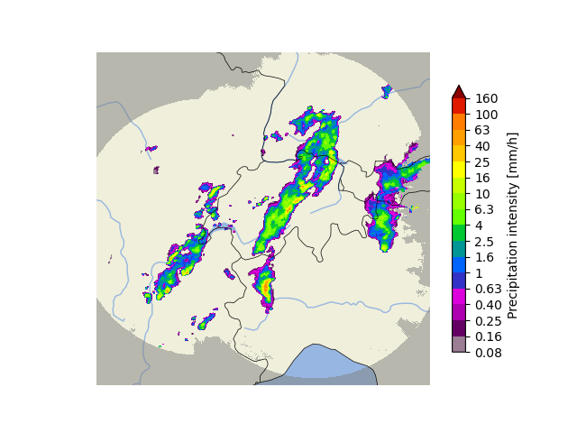
As first step, we need to import the precipitation field that we are going to use in this example.

# Import the example radar composite
root_path = rcparams.data_sources["mch"]["root_path"]
filename = os.path.join(root_path, "20160711", "AQC161932100V_00005.801.gif")
precip, _, metadata = io.import_mch_gif(
    filename, product="AQC", unit="mm", accutime=5.0
)

# Convert to mm/h
precip, metadata = to_rainrate(precip, metadata)

# Reduce to a square domain
precip, metadata = square_domain(precip, metadata, "crop")

# Nicely print the metadata
pprint(metadata)

# Plot the original rainfall field
plot_precip_field(precip, geodata=metadata)
plt.show()

# Assign the fill value to all the Nans
precip[~np.isfinite(precip)] = metadata["zerovalue"]

Out:

{'accutime': 5.0,
 'cartesian_unit': 'm',
 'institution': 'MeteoSwiss',
 'orig_domain': (640, 710),
 'product': 'AQC',
 'projection': '+proj=somerc  +lon_0=7.43958333333333 +lat_0=46.9524055555556 '
               '+k_0=1 +x_0=600000 +y_0=200000 +ellps=bessel '
               '+towgs84=674.374,15.056,405.346,0,0,0,0 +units=m +no_defs',
 'square_method': 'crop',
 'threshold': 0.01155375598376629,
 'transform': None,
 'unit': 'mm/h',
 'x1': 290000.0,
 'x2': 930000.0,
 'xpixelsize': 1000.0,
 'y1': -160000.0,
 'y2': 480000.0,
 'yorigin': 'upper',
 'ypixelsize': 1000.0,
 'zerovalue': 0.0,
 'zr_a': 316.0,
 'zr_b': 1.5}

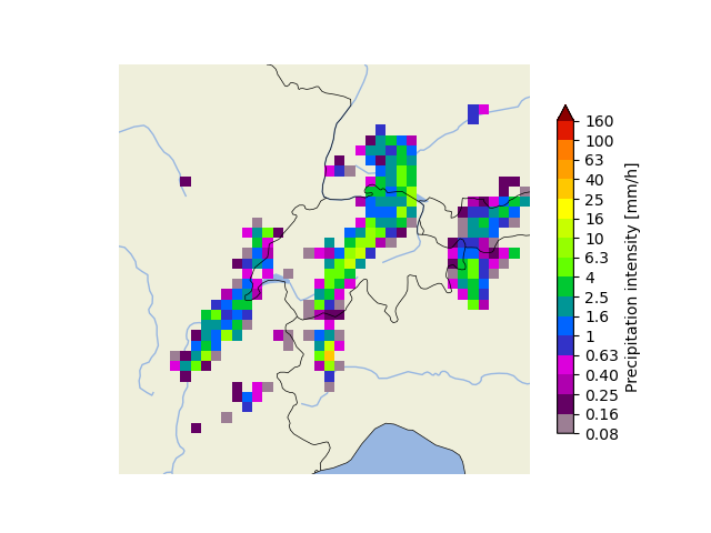
Upscale the field¶

To test our downscaling method, we first need to upscale the original field to a lower resolution. We are going to use an upscaling factor of 16 x.

upscaling_factor = 16
upscale_to = metadata["xpixelsize"] * upscaling_factor  # upscaling factor : 16 x
precip_lr, metadata_lr = aggregate_fields_space(precip, metadata, upscale_to)

# Plot the upscaled rainfall field
plt.figure()
plot_precip_field(precip_lr, geodata=metadata_lr)

Out:

<GeoAxesSubplot:>

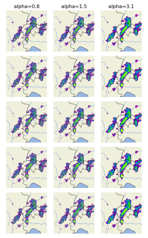
Downscale the field¶

We can now use RainFARM to generate stochastic realizations of the downscaled precipitation field.

fig = plt.figure(figsize=(5, 8))
# Set the number of stochastic realizations
num_realizations = 5

# Per realization, generate a stochastically downscaled precipitation field
# and plot it.
# The first time, the spectral slope alpha needs to be estimated. To illustrate
# the sensitity of this parameter, we are going to plot some realizations with
# half or double the estimated slope.
alpha = None
for n in range(num_realizations):

    # Spectral slope estimated from the upscaled field
    precip_hr, alpha = rainfarm.downscale(
        precip_lr, alpha=alpha, ds_factor=upscaling_factor, return_alpha=True
    )
    plt.subplot(num_realizations, 3, n * 3 + 2)
    plot_precip_field(precip_hr, geodata=metadata, axis="off", colorbar=False)
    if n == 0:
        plt.title(f"alpha={alpha:.1f}")

    # Half the estimated slope
    precip_hr = rainfarm.downscale(
        precip_lr, alpha=alpha * 0.5, ds_factor=upscaling_factor
    )
    plt.subplot(num_realizations, 3, n * 3 + 1)
    plot_precip_field(precip_hr, geodata=metadata, axis="off", colorbar=False)
    if n == 0:
        plt.title(f"alpha={alpha * 0.5:.1f}")

    # Double the estimated slope
    precip_hr = rainfarm.downscale(
        precip_lr, alpha=alpha * 2, ds_factor=upscaling_factor
    )
    plt.subplot(num_realizations, 3, n * 3 + 3)
    plot_precip_field(precip_hr, geodata=metadata, axis="off", colorbar=False)
    if n == 0:
        plt.title(f"alpha={alpha * 2:.1f}")

    plt.subplots_adjust(wspace=0, hspace=0)

plt.tight_layout()
plt.show()

Remarks¶

Currently, the pysteps implementation of RainFARM only covers spatial downscaling. That is, it can improve the spatial resolution of a rainfall field. However, unlike the original algorithm from Rebora et al. (2006), it cannot downscale the temporal dimension.

References¶

Rebora, N., L. Ferraris, J. von Hardenberg, and A. Provenzale, 2006: RainFARM: Rainfall downscaling by a filtered autoregressive model. J. Hydrometeor., 7, 724–738.

# sphinx_gallery_thumbnail_number = 2

Total running time of the script: ( 0 minutes 12.146 seconds)

Gallery generated by Sphinx-Gallery

Precipitation downscaling with RainFARM

Contents